NPV Risk Models
NPV risk modelling is an extension of the basic NPV method in which inputs to the model are allowed to vary so as to represent the effects of risk. The model is run using Monte Carlo simulation. As the inputs vary during the simulation, the output varies in response. After the output values from each of the iterations during the simulation have been collected, the tool operating the model is able to provide an analysis of the project risk, including a risk-based forecast for NPV.
A Simple NPV Risk Model Example
This example has be made as simple as possible so as to illustrate the mechanics of an NPV risk model and how they can be implemented in Excel. It is based on the same project and discount rate as that used for the simple NPV model illustrated on this web site here. Results from the two models can thus be compared.
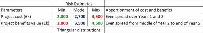
In order to generate inputs to the NPV risk model, the single values for cost and benefits in the simple NPV model are replaced by probability density functions. In this case, the probability density functions are defined using a shape (triangular) and by three point estimates representing the minimum, mode and maximum. The estimates and the apportionment of the related cost and benefits over time are summarised in the table below. Green font denotes best case (optimistic) estimates and red font the worst cast (pessimistic) estimates.
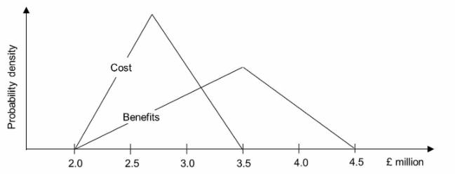
The two probability density functions represent the risk associated with cost and benefits and are illustrated in the figure below. During each iteration of the simulation, a random value selected from the cost probability density function is used to represent the project cost and an independent random value is similarly selected for benefits.
The figure below illustrates how this model can be implemented in Excel. The numbers in brown italics are the risk model input cells; the cells into which randomly varying numbers are injected during the Monte Carlo simulation. The figure illustrates one iteration during the simulation, showing how other cells in italics vary in response to the values simulated in the input cells. A risk tool will use formulae to translate the probability density function associated with each of the risk model inputs into randomly generated numbers. For example the formula to generate numbers for the risk input cell E4 would be:
- Using @RISK for Excel syntax = RiskTriang(B4,C4,D4)
- Using ModelRisk syntax = VoseTriangle(B4,C4,D4)
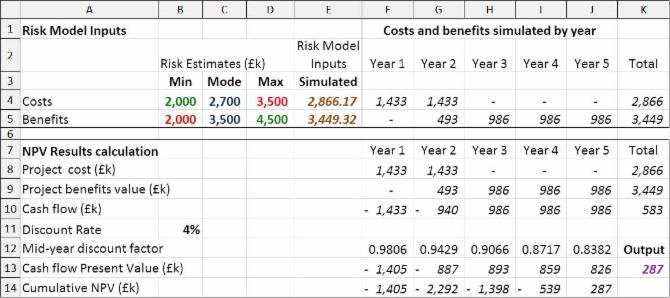
The risk model output is shown in purple bold italics in cell K13. As with the other number in italics, it varies during the simulation in response to the risk inputs. Its values are captured by the risk tool for the purpose of producing the model's results such as those show below (illustrated using a ModelRisk report format).
Excel copies of the model can be downloaded from these links set up to run with either @Risk for Excel or ModelRisk.
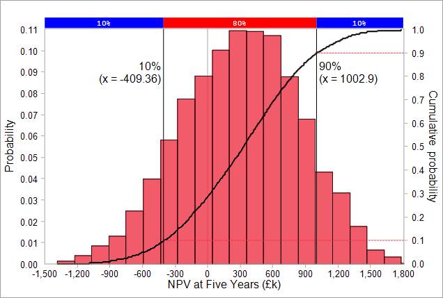
The risk model results above show the risk-based NPV forecasts in two formats:
- histogram (in this case using 20 intervals) and
- cumulative probability graph (s-curve)
The risk modelling tool provide a variety of statistical results. For the above case, these results include:
- mean NPV = £310k;
- median NPV = £330k;
- NPV standard deviation = £540k;
- skewness = -0.11;
- probability of NPV = greater than zero, approximately 72%;
- probability of NPV = less than zero, approximately 28%.
Notes
The actual results when you run the model may vary slightly from these results. There will also be a degree of random variation from one run of the model to the next unless the same simulation seed is used.
Skewness in the results is a consequence of skewness in the probability density functions for cost and benefits of which skewness in the latter is the pronounced.