Correlating Risk Model Inputs
In a simple Monte Carlo model, the randomised outcome for each risk model input is simulated as being independent of the randomised outcome for the other inputs. In practice, this usually unrealistic. In real projects, we find that risks are affected by interrelationships that result in covariance between their outcomes. Correlating risk model inputs is a modelling technique that adjusts the simulation process to reflect the implications of covariance.
Why does Covariance Occur on Projects?
Covariance between risk model inputs may be appropriate as a consequence of causal links between them, the influence of common factors or a combination of both.
Causal links can exist as a consequence of dependencies between associated activities. For example, on a construction project in which the sponsoring organisation has employed a design company and a building company, the two company's activities will be linked in a multitude of ways. Both, for example, might be able to increase costs as a consequence of requirement changes. Where causal links exist, there is usually a strong case for believing that there will be covariance between outcomes. This can be simulated by introducing a positive correlation between the associated risk model inputs.
The existence of common factors that influence activity outcomes is often a broader cause of covariance. As a minimum, the effectiveness with which a project is managed is liable to have a common influence. Schedule risk may also be an important common factor that affects inputs to an NPV risk model.
Introducing Correlation to Risk Model Inputs
Risk tools such as @RISK for Excel and ModelRisk allow risk model inputs to be correlated using one or more correlation matrices. The figure below is an example of a correlation matrix and is used to model covariance between risk model cost inputs.
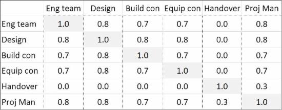
The numbers in the matrix represent coefficients of correlation. The coefficient of correlation is zero if there is no relationship between a pair of risk inputs. Positive correlation is simulated with coefficients between zero and one, with 1.0 representing perfect positive correlation.
Effect of Introducing Correlation
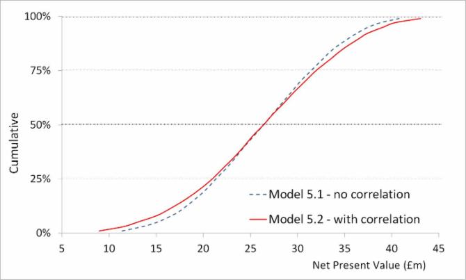
The figure below illustrates the typical effect of introducing positive correlation to the risk inputs for either costs or benefits in an NPV risk model: the range of forecast results is broadened, with the most difference being made to the output distribution tail ends. It has been produced by running Model 5.1, which has no correlation and Model 5.2, which uses the above correlation matrix, but which is otherwise identical. The models can be downloaded from this page.
Notes
- The broadening of the results curve shown above is relatively small compare to many models. In general, correlation becomes more important as the number of risk model increases.
- Since any correlation matrix has mirror symmetry around the diagonal from the top left corner to the bottom right, its values only need to be entered in one half of the matrix when populating cells in a risk tool.
- A matrix may be invalid if the effects of certain combinations of correlation coefficients cannot be simulated. A good risk tool will include a function that adjusts the matrix to the nearest valid one. Both @RISK for Excel and ModelRisk have this capability.
- There is sometimes a case for introducing negative coefficients of correlation. For example, increased costs might be associated with decreased benefits.
- Introducing correlation to inputs affects risk prioritisation results produced by the cruciality and conditional mean techniques described on this page. When producing prioritisation results, the best approach is usually to run a version of the model without correlation.